On the Magnetosphere-Ionosphere Coupling During the May2021 Geomagnetic Storm

On 12 May 2021 the interplanetary doppelgänger of the 9 May 2021 coronal mass ejection impacted the Earth’s magnetosphere, giving rise to a strong geomagnetic storm. This paper discusses the evolution of the various events linking the solar activity to the Earth’s ionosphere with special focus on the effects observed in the circumterrestrial environment. We investigate the propagation of the interplanetary coronal mass ejection and its interaction with the magnetosphere—ionosphere system in terms of both magnetospheric current systems and particle redistribution, by jointly analyzing data from interplanetary, magnetospheric, and low Earth orbiting satellites. The principal magnetospheric current system activated during the different phases of the geomagnetic storm was correctly identified through the direct comparison between geosynchronous orbit observations and model predictions. From the particle point of view, we have found that the primary impact of the storm development is a net and rapid loss of relativistic electrons from the entire outer radiation belt. Our analysis shows no evidence for any short-term recovery to pre-storm levels during the days following the main phase. Storm effects also included a small Forbush decrease driven by the interplay between the interplanetary shock and subsequent magnetic cloud arrival.

On 12 May 2021 a coronal mass ejection (CME) emitted from the Sun on 9 May 2021 impacted the Earth, giving rise to a strong geomagnetic storm. This paper present a global view of the CME effects observed in the circumterrestrial environment focusing on its propagation and on its interaction with the magnetosphere—ionosphere system in terms of both magnetospheric current systems and particle redistribution, by jointly analyzing data from interplanetary, magnetospheric, and low Earth orbiting satellites. The principal magnetospheric current system activated during the different phases of the geomagnetic storm was correctly identified through the direct comparison between geosynchronous orbit observations and model predictions. From the particle point of view, we have found that the primary impact of the storm development is a sudden loss of relativistic electrons from the entire outer radiation belt. Such kind of a global analysis is still the straightforward way available to understand the complex dynamics of the processes occurring in the circumterrestrial environment from a space weather point of view.

Geomagnetic storms and substorms are among the most important signatures of the variability in the solar-terrestrial relationship. They are extremely complicated processes, which are triggered by the arrival of solar perturbations, such as interplanetary coronal mass ejections (ICMEs), solar flares, co-rotating interaction regions (CIRs), etc. (e.g., Gonzalez et al., 1994; Gosling et al., 1990; Knipp, Delores J. et al., 2021; Miyake et al., 2019; Piersanti et al., 2020). These processes, involving a wide range of plasma regions and phenomena which mutually interact with both the magnetosphere and ionosphere, are usually non linear. For the last 30 years, numerical simulations, and both ground-based and space-borne observations have been highlighting such a strong feedback and coupling process (Hayakawa et al., 2020; Navia et al., 2018; Piersanti et al., 2020; Reyes et al., 2019, and references therein). On this topic, the space weather scientific community started more and more to conduct comprehensive analysis on several “famous geomagnetic storm past events” (Boteler, 2019; Cliver Edward & Dietrich William, 2013; Hayakawa et al., 2019; Hayakawa, Hattori, et al., 2021; Knipp et al., 2018) trying to understand why extreme solar-terrestrial storms occasionally form perfect storms (Y. D. Liu et al., 2019). Those are the reasons why, in order to properly understand geomagnetic storms and substorms, it is necessary to consider the entire chain of events as a single process. When solar perturbations are analyzed, one has always to consider that the dynamic pressure of the solar wind (SW) and the interplanetary magnetic field (IMF) control the strength and the spatial structure of the magnetosphere-ionosphere current systems. The changes of these current systems are at the origin of geomagnetic activity, and consequently of the variation in the Earth’s magnetospheric-ion ospheric field as observed by space-borne and ground-based instruments. Indeed, a significant amount of solar wind plasma can be dropped off either directly in the polar ionosphere (polar cusp and cap) or stored into the equatorial central regions (central plasma sheet, current sheet, etc.) of the Earth’s magnetospheric tail, from where it is later injected into the inner magnetospheric regions, such as the radiation belts (RBs) (Gonzalez et al., 1994), which are a pair of toroidal regions around the Earth, that are filled with magnetically-entrapped charged particles of high energy. The growth of the trapped particle population in the inner magnetosphere produces a significant increase of the ring current, while the energy released from the magnetotail and injected into the high-latitude ionosphere, together with that directly deposited in the polar regions, is responsible for an enhancement of the auroral electrojet current systems (Kivelson et al., 1995). The importance of studying these processes lies not only in the understanding of the physical processes that characterize the solar-terrestrial environment, but also in their impact on technological systems both at ground and in space, not to mention risks to human health (e.g., A. Pulkkinen et al., 2017; Baker et al., 2016; Carter et al., 2016; Dyer et al., 2018; Lanzerotti, 2001, 2017; Plainaki, Christina et al., 2020; Riley et al., 2018). Space Weather can indeed impact space-based and terrestrial technological infrastructures. Sporadic events, such as geomagnetic storms, can influence satellite and payload functions, and (in extreme cases) they can even cause the loss of a mission. In fact, a large fraction of space systems operates at altitudes of a few hundred to a few ten thousand km above the Earth’s surface, in the region of the Van Allen RBs. In the Van-Allen-Probes (VAPs) Mission era, spanning the 2010s, the MagEIS and the REPT instruments on board the VAPs (Baker et al., 2013; Blake et al., 2013) returned a detailed picture of particle populations in the belts and their dynamic rearrangement triggered by solar forcing. Especially the outer radiation belt (ORB), which is dominated by energetic electrons up to several MeV, is heavily affected by geomagnetic disturbances, while the intermediate slot region, relatively devoid of electrons in quiet period due to pitch-angle scattering, can be subject to sudden refilling during strong storms (Baker et al., 2018, and references therein). On the other hand, it has been proven that the relativistic electron injection into the inner radiation belt (IRB), which is dominated by high-energy protons, is hindered by an “impenetrable barrier” at ∼2.8 RE, except for a short transient during the Halloween storm of 2003 (Baker et al., 2014).

Furthermore, it has been found that the efficiency of electron acceleration is primarily influenced by the IMF orientation and solar wind speed and dynamic pressure, and mostly achieved via resonant wave-particle interactions with VLF chorus waves (Koskinen et al., 2017; W. Li et al., 2014).

In this paper, we offer a global analysis of the 12 May 2021 geomagnetic storm, which represents a great space weather event occurring a few years after a new solar cycle onsets. We want to highlight here that despite statistical studies showed that strong geomagnetic storms take place around the maximum and in the declining phase of solar cycles (Meng et al., 2019, and reference therein), even under quiet Sun conditions significant space weather events can occur (Garcia & Dryer, 1987; Hayakawa et al., 2020; Hayakawa, Schlegel, et al., 2021; Willis & Stephenson, 2000). So the 12 May 2021 represents a significant case whose global analysis could help the current understanding about the direct link between solar driver and the relative geomagnetic response.

The paper is organized as it follows: Section 2 presents the analysis of the CME propagation in the interplanetary space; Section 3 shows the magnetosphere-ionosphere analysis; Section 4 includes the discussion and conclusions.

2.1. CME Lift-Off and Interplanetary Response

The CME was visually identified as a diffuse plasma structure both on STEREO-A SECCHI-COR2 and SOHO LASCO C2 FoVx (Field of Views). It enters COR2 FoV on 9 May 2021 at 11:40 UT ±30 min and reaches the FoV edge on 9 May 2021 at 15:40 UT ±30 min, with an estimate PoS (Plane of Sky) velocity VPoS = 600 ± 100 km/s. It enters LASCO C2 FoV on 9 May 2021 at 14:30 UT ±30 min and reaches the FoV edge on 9 May 2021 at 16:00 UT ±1 hr, with an estimate PoS velocity VPoS = 550 ± 100 km/s. The angle subtended by the Earth, Sun, and Stereo-A on that day was very close to 45° (see Figure 2), and subsequent observations by HI-1, which imaged the CME at a larger distance from the Sun allowed us to obtain another estimate of the ICME PoS velocity: The ICME crossed HI-1 FoV from the early hours of 10 May 2021 to late 11 May 2021 with an estimate PoS velocity of 500 km/s, obtained via the time-elongation fitting method (Barnes et al., 2019).

The most probable source for the CME was a filament eruption observed on 9 May 2021 at t0 = 11:30 UT in the southern solar hemisphere (white cross in Figure 1). The filament ejection has been recorded by SDO AIA (Lemen et al., 2012; Pesnell et al., 2011) imagers. At the time of the CME lift-off, a large coronal hole (CH—Gray line in Figure 1) was present in close proximity of the filament coordinates. The CH was likely associated to a fast solar wind stream affecting the CME propagation. Considering the source on the Sun and the hypothesis of radial propagation, we can de-project the CME PoS velocities and estimate its radial velocity as Vrad = 720 ± 100 km/s. Also, hypothesizing a cone shape for the CME and a self-similar expansion, the width of the CME can be estimated to be 50° ± 5°.

To describe the ICME propagation in the heliosphere we have used the P-DBM (Del Moro et al., 2019; Napoletano et al., 2018) model. This model assumes that the ICME dynamics is governed only by its interaction with the ambient SW. By employing a fluid dynamic analogy, the force acting on the ICME depends on the square of the ICME velocity relative to the ambient SW flow, such that the equation for the ICME radial acceleration reads:

aa = −γγ(rr) [vv − ww(rr)] |vv − ww(rr)|

where γ(r) is the so-called drag parameter representing the interaction efficiency between the ICME and the SW, w(r) is the SW speed, v is the ICME speed, and r is the distance from the Sun. A good approximation beyond 20 solar radii is obtained assuming that γ and w are constant throughout the whole ICME propagation (Cargill, 2004; Vršnak et al., 2013). Under such assumptions, Equation 1 can be solved analytically providing the temporal evolution of the ICME’s heliospheric distance and velocity. The P-DBM model includes in this framework the uncertainties on the initial ICME parameters and on the actual γ and w values, by means of a Probability Distribution Function and a Monte-Carlo like approach (see a detailed description in Napoletano et al., 2018, 2021). Our conjecture is that the part of the ICME hitting the Earth interacted with the fast SW generated by the CH over the whole duration of its travel, and, consequently, we have estimated its time to travel to 1AU and its velocity at arrival. From 10,000 runs of the P-DBM model, the obtained ICME’s arrival time and velocity at 1AU are: t1AU = 2021-05-12 04:00 ± 6h and V1AU = 640 ± 70 km/s. As evident from the propagation scheme reported in Figure 2, the ICME did not hit any relevant interplanetary spacecraft, nor any inner other Solar System planet.

Figure 3 shows the passage of the ICME as observed by the Wind (Lepping et al., 1995) spacecraft located at the first Lagrangian point. On 12 May 2021 at ∼05:55 UT, the spacecraft detected a clear interplanetary shock (IPs—Red dashed line on the left panels), characterized by a large increase in the SW density (Δnp,W ≈ 38 cm−3, panel a), velocity (ΔvSW,W ≈ 120 km/s, panel b) and dynamic pressure (ΔPSW,W ≈ 11 nPa, panel c), as well as in the IMF strength (ΔBIMF,W ≈ 8 nT, panel d). Using the Rankine-Hugoniot conditions, under the assumption that both energy and momentum are conserved across the shock front (Landau et al., 1960; Oliveira, 2017), we have estimated the shock normal, obtaining the following orientation: ΘSE,W = 177° ± 5° and ΦSE,W = 111° ± 5° (ΘSE,W and ΦSE,W being the angles formed by the shock normal with the Sun-Earth line and with the y axis in the yz plane, respectively (Xu et al., 2020)). In addition, we have estimated the shock speed as vsh,W = 538 km/s ± 10 km/s. The propagation of the IPs plane from WIND to the Earth’s magnetopause is represented in Figure 3h using red dotted lines. From such results, under the assumption of planar propagation along the direction marked by the black arrow in Figure 3h, we have predicted both the time and location of the IPs impact onto the magne-

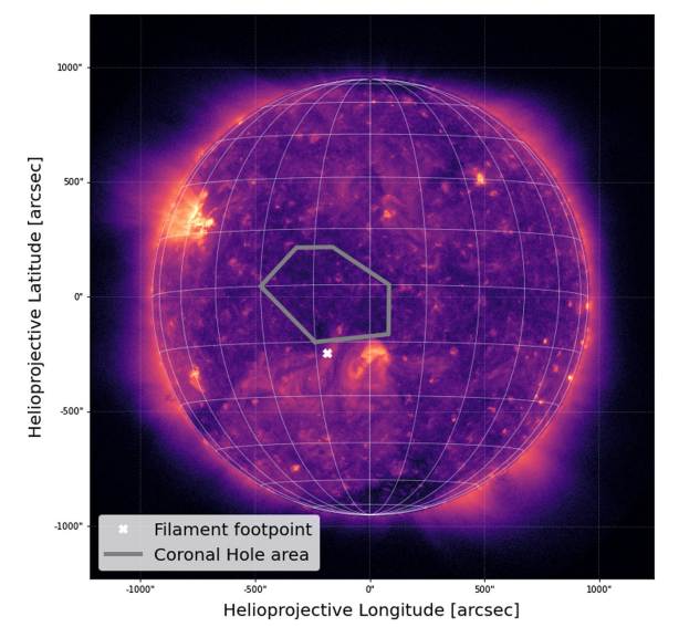
Figure 1. EUV image of the Sun by solar dynamics observatory AIA211 at the time of the filament eruption. The white cross marks the position of the filament eruption associated with the coronal mass ejection; the gray line marks the position of the coronal hole.

tosphere (green rectangle in Figure 3h), obtaining 06:34 UT (i.e., 37 min after WIND observations) and 12:49 (±00:15) LT (i.e., in the noon sector of the magnetosphere), respectively.

The 12 May 2021 ICME was characterized by a significant magnetic cloud observed between ∼07:36 UT and ∼15:24 UT. Its boundaries have been determined according to the the magnetic field behavior together with temperature, velocity and density of solar protons (Burlaga et al., 1981), as depicted in the blue shaded region of Figure 3 (left panel). Indeed, plasma temperature decreases from ∼1.7 ⋅ 10^5K to ∼6 ⋅ 10^4K (not shown), SW speed remains almost constant at ∼480 km/s for about 8 hr (panel b), and the total magnetic field increases to 22 nT (panel d) with a smooth, pronounced and prolonged (approximately 4 hr) southward rotation at ≈11:30 UT (panel g).

The storm’s main phase was followed by short-lasting substorm activity, as highlighted by |AL|-index values which dropped back to <300 nT just after 6 hr from the occurrence of Dst minimum. This activity is likelyntriggered by suitable IMF preconditions (Tsurutani & Zhou, 2003), consisting in ∼3 hr of steadily southward vertical field component upstream of the IPs.

This section is dedicated to the investigation of the magnetospheric-ionospheric system during the 12 May 2021 geomagnetic storm. An accurate knowledge of the magnetosphere-ionosphere coupling dynamics, in terms o magnetospheric-ionospheric current systems and particle distribution function (A. Lui et al., 2000; Consolini & De Michelis, 2005; Milan et al., 2017; Sitnov et al., 2001), in response to the variations of the SW conditions (magnetic field orientation, plasma density, velocity, etc.) is crucial in many sectors of space weather.

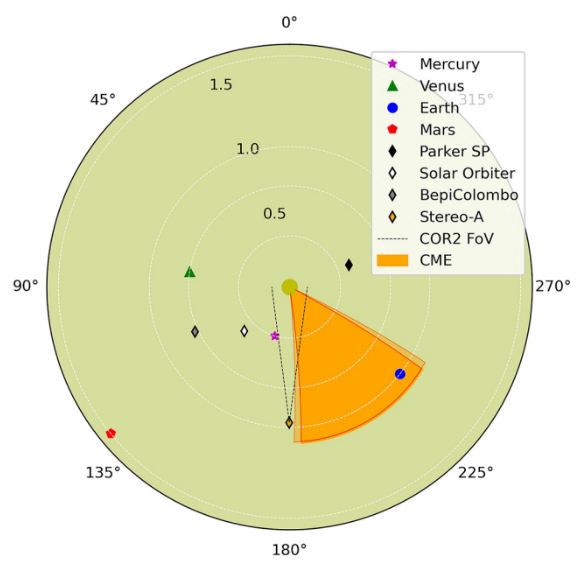
Figure 2. Geometrical properties for the propagation of the coronal mass ejection (CME) in the inner heliosphere. The positions of the inner planets and relevant spacecrafts are represented by colored symbols. The interplanetary coronal mass ejection (ICME) is represented by the orange shadowed area. The lighter orange area represent the 1σ uncertainty about the ICME position from the P-DBM runs.

3.1. Magnetosphere

Figure 4a shows the response of the magnetosphere to the arrival of the interplanetary shock. According to the Shue et al. (1998) model, the magnetopause nose moved back to ∼6.8RE. Indeed, the shapes of the magnetospheric field lines before (black lines) and soon after (red lines) the IPs, evaluated by means of the TS04 model (Tsyganenko & Sitnov, 2005), show a large field compression. Correspondingly, on May 12 at ∼6:35 UT, GOES 16 (Figure 4b, left column; LTG16 = UT − 5) and GOES 17 (Figure 4b, right column; LTG17 = UT − 9.1) measured a sudden variation (Δt ∼ 10 min) in the north-south component of the magnetic field (ΔBz,G16 = −28 nT and ΔBz,G17 = 18.8 nT), due to the compression of the magnetosphere, coupled with a stretching of the magnetotail field lines (ΔBx,G16 = 22 nT and ΔBx,G17 = 14.6 nT), caused by the concurring contribution of the IPs impinging onto the magnetopause and of the southward switching of the IMF (Piersanti et al., 2020; Piersanti & Villante, 2016; Villante & Piersanti, 2011).

A different situation is visible between May 12 at ∼11:36 UT and May 12 at ∼15:24 UT, corresponding to the arrival of the magnetic cloud. During such time interval, GOES 16 and GOES 17 were located at 06:36 < LTG16 < 10:24 and 02:36 < LTG17 < 06:24, respectively. In the morning side, GOES 16 observed a huge double peaks decrease along all the magnetic field components (Figure 4b, left panels). In the nighside, GOES 17 showed positive variations in both Bx and By components (Figure 4b, top and mid right panels), and large double peak increase along Bz (Figure 4, bottom right panel). This behavior is the signature of a strong stretching and twisting of the magnetospheric field lines and can be interpreted in terms of the concurring contribution of the partial ring current intensification and of a magnetotail current reshaping (Kalegaev et al., 2005; Ohtani et al., 2007; Piersanti et al., 2020; T. I. Pulkkinen et al., 2006). Such a scenario is confirmed by the direct comparison between a modified TS04 model (hereafter TS04*) marked by red dashed lines in Figure 4, in which we considered the contribution of the ring current and tail current (hereafter, TC) alone during the geomagnetic storm. It can be easily seen that the TS04* trace gives a good representation of the behavior of the GOES observations, confirming the key role of the ring current in the morning sector of the magnetosphere and of the tail current in the nightside sector of the magnetosphere (e.g., Kalegaev et al., 2005; Ohtani et al., 2007, and reference therein). We need to underline here that in order to have the best model representation of the magnetospheric field observations, the principal parameters of the TC in the TS04 model was customized in the following way: the hinging point RH (defining the position of the plasma sheet bending, separating the rigidly tied near-Earth part from the more distant tailward plasma sheet) has been shifted from 8.75RE to 6.85RE (Dayeh et al., 2015; Tsyganenko & Sitnov, 2005; Xiao et al., 2016); the current sheet thickness DH has been changed from 5RE to 5.9RE (Kan, 1973; Thompson et al., 2005; Tsyganenko & Sitnov, 2005). From a pure physical point of view, the passage of the magnetic cloud caused both a magnetospheric dipolarization and an intensification of the plasma density in the magnetotail neutral sheet, leading to a change in RH and an increase of DH, respectively (A. T. Y. Lui, 2016; Murphy et al., 2022, and reference therein). The largest discrepancies between GOES measurements and TS04* predictions occurred at the peak of the main phase. Such discordance might be related to the fact that the Tsyganenko & Sitnov (2005) model estimated, at the

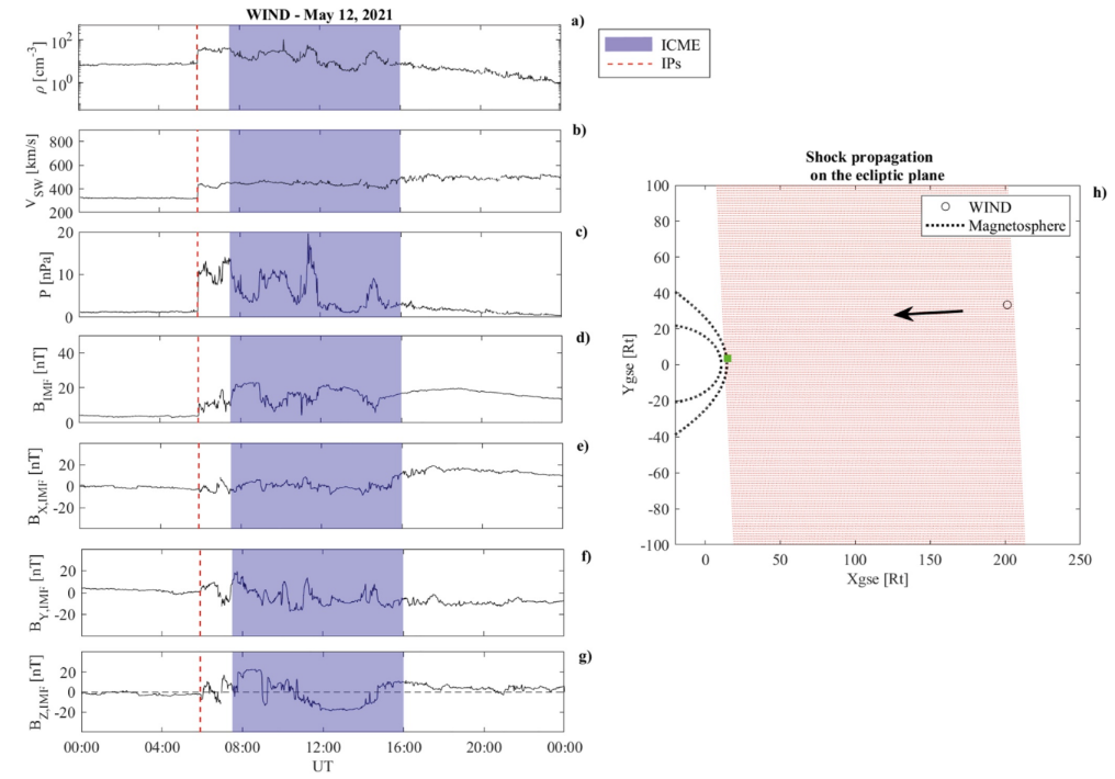
Figure 3. Solar wind parameters observed by the WIND spacecraft at L1: (a) Proton density; (b) velocity; (c) dynamic pressure; (d) interplanetary magnetic field (IMF) intensity; (e–g) IMF components (BX,IMF, BY,IMF, BZ,IMF respectively) in the GSE reference frame. The red dashed line marks the interplanetary shock as observed on 12 May at ≈5:56 UT. The blue shaded region identifies the magnetic cloud; (h) Interplanetary shock propagation in the ecliptic plane. Here red dotted lines represent the shock plane propagation in the ecliptic plane and the arrow its direction. The green rectangle represents the estimated impact position of the IPs onto the magnetopause.

peak of the main phase, a backward motion of the magnetopause up to 6.2RE, which is behind the GOES satellite orbit.

3.2. Ionosphere

Figure 5a shows CSES (China Seismo Electromagnetic Satellite) (Shen et al., 2018) magnetic observations (Zhou et al., 2019) along the North-South (BN – left panel), East-West (BE—Central panel) and Vertical (BC—Right panel) direction, respectively, from 11 May to 14 May 2021, after removing the internal and crustal contributions to the Earth’s magnetic field by use of the CHAOS-7 model (Finlay et al., 2020). CSES is a Chinese satellite launched on 2 February 2018, hosting a fluxgate magnetometer, two Langmuir probes, an electric field detector and two particle detectors out of eight payloads. The satellite orbits at about 500 km of altitude (Low Earth Orbit – LEO) in a quasi-polar Sun-synchronous orbit, and it passes at about 02:00 and 14:00 local time (LT) in its ascending and descending orbits, respectively (Shen et al., 2018).

As expected (Villante & Piersanti, 2011), the action of both the magnetospheric and ionospheric currents produced largest variations along BN,Magn and BE,iono, respectively.

In order to quantify the contributions of magnetospheric and ionospheric origin at CSES orbit, we have applied the MA.I.GIC. model (Piersanti et al., 2019) to discriminate between different time scales in a time series. Results are shown in Figure 5b. Upper and lower panels report observations of high (∼22.3 μHz < f < ∼2.8 mHz; f being the

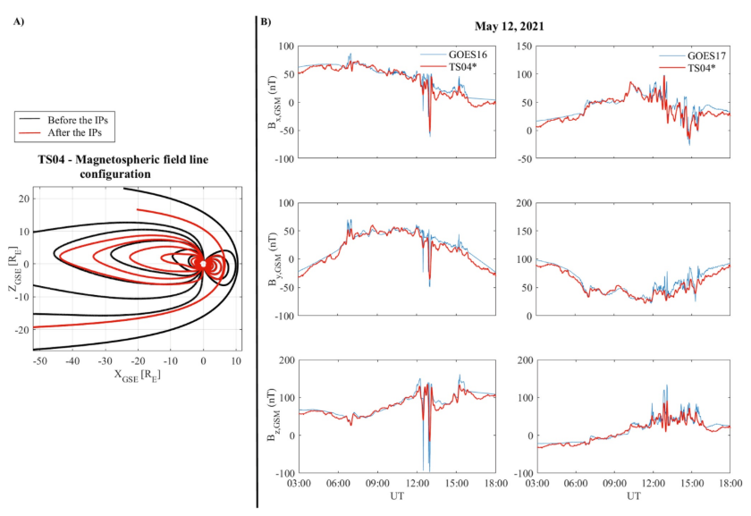
Figure 4. (a) TS04* model prediction of the magnetospheric field lines configurations before (black lines) and after (red lines) the passage of the interplanetary shock; (b): Magnetospheric field observations along XGSM (upper panels), YGSM (middle panels) and ZGSM (lower panels) at GOES 16 (LT = UT-5) and GOES 17 (LT = UT-9) geosynchronous orbit; red dashed lines represent the TS04*+IGRF model predictions.

frequency) and low frequency (∼2.6 μHz < f < ∼21 μHz) components, respectively. The low frequency behavior shows a strong and rapid decrease along the North-South direction during the main phase of the geomagnetic storm, and a long lasting increase during the recovery phase. On the other hand, BE,LF and BC,LF show a negligible/null variation over the entire period under analysis. This behavior is consistent with field variations of magnetospheric origin induced by the action of both the asymmetric part of the ring current and tail current along BN,LF (Lühr & Zhou, 2020; Neubert et al., 2001; Park et al., 2020). This scenario is confirmed by the comparison between the CSES contribution of magnetospheric origin and TS04* model (red lines in Figure 5, bottom row). It can be easily seen that the TS04* model well represents the variations along BN,LF, BE,LF and BC,LF.

The high frequency components, instead, show large variations along BE,HF. This behavior is consistent with contri-butions due to both the variations in the ionospheric-current system and magnetospheric-ionospheric coupling processes (e.g., field aligned current contribution). Indeed, the positive then negative variations observed in the horizontal plane during the main phase can be ascribed to the loading-unloading process between the magnetosphere and ionosphere (Consolini & De Michelis, 2005; Piersanti et al., 2020), while, the huge positive variations observed during the recovery phase can be due to the ionospheric DP-2 current system (Kamide, 1988; Kamide et al., 1997; Piersanti & Villante, 2016; Villante & Piersanti, 2011).

In order to evaluate the rearrangement of electron populations in the Earth’s magnetosphere, we have applied an approach analogous to the one reported in Palma et al. (2021) for the 26 August 2018 geomagnetic storm, using particle data from the MEPED-90° electron telescope on board the NOAA19-POES satellite (Evans & Greer, 2004) and the High-Energy Particle Detector (HEPD-01) on board the CSES satellite (Picozza et al., 2019). The NOAA19-POES is Sun synchronous nearly-polar satellite orbiting at LEO altitudes. NOAA19 is currently orbiting at an altitude of ∼850 km with a 98.7° inclination and an orbital period of ∼102 min. In both cases, to

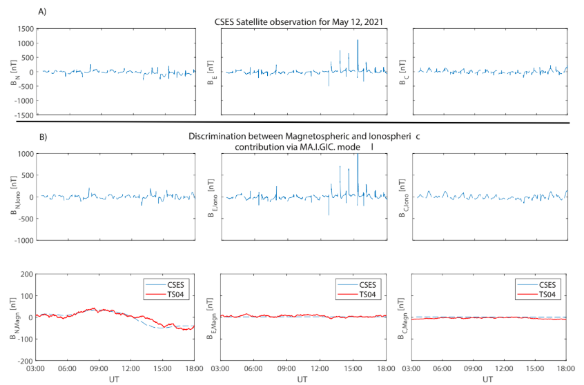
Figure 5. (a) HPM observations, for 12 May 2021, at Low Earth Orbit along geographic North-South (left panel), East-West (middle panel) and vertical (right panel) components; (b) Application of the MA.I.GIC. model to HPM data: Top panels show the contribution of ionospheric origin (∼22.3 μHz < f < ∼2.8 mHz; f being the frequency time scale) for the three components of the observed field; lower panels show the contribution of magnetospheric origin (∼2.6 μHz < f < ∼21 μHz) for the three components of the observed field. Red lines represent the TS04* model previsions.

avoid saturation or pile-up issues possibly occurring at extremely high particle rates, the South Atlantic Anomaly has been excluded by means of a cut in the available geomagnetic-field values (no B-values lower than 23,000 nT). Figure 6b) depicts the behavior of MEPED integral electron fluxes over the >0.13 MeV range as a function of the McIlwain L parameter (McIlwain, 1961) throughout the pre-storm, storm, and recovery phases. The flux values, which are dominated by the contribution of low-energy electrons (Turner et al., 2015), point out a prolonged slot-filling event immediately downstream of maximum geomagnetic disturbance, characterized by flux enhancements by a few orders of magnitude. Correspondingly, the plasmapause (full black line), estimated from the X. Liu and Liu (2014) model, steps back to L ∼ 3.8.

It is worth noticing that measurements taken in the Van-Allen-Probes era on the occasion of multiple CME-driven storms associated with IP shock compressions (Khoo et al., 2018) have established a spatial and temporal correlation between plasmapause location and the initial enhancement of energetic electrons over an energy range pretty close to the one spanned by the MEPED electron telescope in Figure 6b). At the onset of 12 May 2021 storm, the concurrent substorm activity may represent a suitable candidate for the injection of such source/seed populations to be resonantly accelerated by ULF waves at the boundary of the plasmasphere, where the plasma density gradient affects wave growth (W. Liu & Cao, 2014) and interactions.

Panels (c and d) in Figure 6 contain MEPED fluxes over the >0.65 MeV range and the rate of >4.5 MeV particles detected by HEPD-01,respectively. At L shells typical of the ORB, a persistent depletion starts right after the onset of the main phase, with no short-term flux recovery to pre-storm levels (Palma et al., 2021, and reference therein). These ORB losses in the relativistic range may be consistent with magnetopause shadowing (Herrera

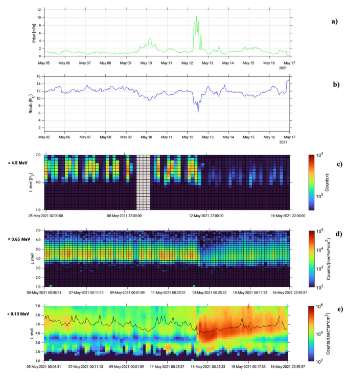
Figure 6. Panel (a): Time profile of the solar wind dynamic pressure (OMNI data magenta curve) and position of the magnetopause standoff distance (as estimated from the Shue et al. (1998) model, black curve) over the period of 5–16 May 2021; Panel (b): >0.13 MeV electron fluxes measured by MEPED-90° over the same period. The superimposed black line represents the position of the plasmapause as estimated from the X. Liu and Liu (2014) model; Panel (c) >0.65 electron fluxes measured by the azimuthal MEPED-90° telescope on board the NOAA19 satellite over the same period; Panel (d): Rates of >4.5 MeV particles detected by High-Energy Particle Detector (HEPD-01) over the same period. Gray shaded areas refer to time intervals for which HEPD data are not available.

et al., 2016) and outward radial transport, as suggested by a deep incursion of the magnetopause, as estimated from the Shue et al. (1998) model, on L shells no higher (Case & Wild, 2013) than ∼6.2 RE in correspondence with the peak of the storm (Figure 6a). Further considerations about the role of magnetopause shadowing in the May 2021 storm event are reported in Section 4.

Figure 7. 12-hr averaged galactic cosmic-ray (GCR) proton intensity variation profile as a function of time from High-Energy Particle Detector (HEPD-01) observations in the >150 MeV energy range (top panel). A clear suppression of GCR intensity can be spotted after 12 May 2021 0600 UTC. At the same time, it is possible to see an abrupt variation in Dst index (bottom panel).

Forbush decreases (FDs) refer to sudden suppression of the short-term galactic cosmic-ray (GCR) intensity (Forbush, 1937; Hess & Demmelmair, 1937), either associated with corotating high-speed streams (“recurrent” FDs) or caused by transient solar wind structures following coronal mass ejections from the Sun (“non-recurrent” FDs). Most of the early observations of such phenomena were carried out by ground-based detectors, such as Neutron Monitors and Muon Telescopes (Cane, 2000; Papailiou et al., 2020; Vieira et al., 2012), and by measurements with ionization chambers (Hayakawa, Oliveira, et al., 2021) allowing only for an indirect detection of the neutrons generated in the atmosphere. Figure 7 shows the variation of GCR protons measured by the HEPD 01 instrument, directly from space, across the storm and post-storm of May 2021. The 12-hr-averaged galactic protons intensity variation as a function of time has been studied in the >150 MeV energy range (red points in the top panel), selecting only particles at the very polar sectors of the CSES-01 orbit, where the geomagnetic cutoff is low enough to allow, in the absence of strong proton events (e.g., Piersanti et al., 2017; Tranquille, 1994), for galactic proton detection. The applied selection criteria were the same described in Bartocci et al. (2020). A clear suppression of GCR intensity after 12 May 2021 0600 UTC is evident, in conjunction with the arrival of the storm, as observed by the abrupt variations in Dst index (bottom panel). The overall maximum variation of the proton intensity profiles is around −10%.

The observations of cosmic ray variation during solar flares or CMEs provide constraints on the acceleration mechanisms and magnetic reconnection processes operative in the flares. CMEs and the shocks they drive cause FDs, and since the same phenomena are also responsible for geomagnetic storms, the study of the time-profiles of GCRs during such storms could provide valuable information about these space weather disturbances. Furthermore, certain phenomena associated with FDs, such as precursory decreases and spatial anisotropies can give advanced information regarding the intensity of geomagnetic storms themselves. For this reasons, it is important to have a detector that can study even small FDs (like the one reported in this work) with a sufficient precision and directly from space.

The 12 May 2021 geomagnetic storm was caused by a CME occurred on 9 May 2021 at t0 = 11:30 UT as a consequence of a filament eruption observed in the southern solar hemisphere, as recorded by SDO AIA imagers. Under the hypothesis of radial propagation, and de-projecting the CME velocity, we have estimated its radial velocity as Vrad = (720 ± 100) km/s. Observations by HI-1 confirmed such results, by imaging of the ICME at a larger distance from the Sun from the early hours of 10 May 2021 to late 11 May 2021 with a PoS velocity of 500 km/s. It is interesting to note that, at the moment of the CME lift-off, a large CH (gray line in Figure 1) was present very close to the filament coordinates, leading to fast SW stream that very likely affected the CME propagation in the interplanetary space.

To reproduce the ICME behavior in the interplanetary space, we have used the P-DBM (Napoletano et al., 2018) model for the propagation of the CME in the heliosphere. Under the hypothesis that the part of the ICME hitting the Earth interacts with the fast SW generated by the CH over the whole duration of its travel, we have estimated its time travel to 1AU and its velocity at arrival, obtaining 12 May 2021 at 04:00 ± 6h and 640 ± 70 km/s, respectively. Such estimations are confirmed by the observations at the first Lagrangian point (WIND satellite), which detected the ICME arrival on May 12 at 08:23 UT. The magnetic cloud was preceded by an interplanetary shock passing through the satellite at 05:56 UT. We have estimated both the shock normal orientation as ΘSE,W ≈ −177° and ΦSE,W ≈ 111°, and the shock speed as vsh,W ≈ 538 km/s. Under the assumption of a planar propagation, we have obtained that the IPs impacted onto the magnetopause in the noon sector.

The consequence of the ICME passage through the Earth’s magnetosphere was the reconfiguration of the magnetospheric principal current systems. At the moment of the arrival of the IPs, the magnetopause nose moved back to ∼6.8 RE, as a consequence of the concurrent contributions of a strong increase in the SW dynamic pressure and the southward switching of the IMF orientation (Lee & Lyons, 2004; Piersanti et al., 2020; Piersanti & Villante, 2016; Villante & Piersanti, 2011; Wang et al., 2009). As to the magnetospheric field observed at geosyn-chronous orbit, strong variations in both BZ,GSE and BX,GSE were detected. During the passage of the magnetic cloud, the magnetospheric field lines turned out strongly stretched and twisted. Indeed, geosynchronous observations showed: (a) a huge decrease along both the Bz,GSE and Bx,GSE in the local morning sector (06 : 36 < LTG16 < 10 : 24); (b) an increase then decrease along Bz,GSE coupled with a large decrease in both Bx,GSE and By,GSE components in the local night sector (02:36 < LTG17 < 06:24). We interpreted those observation as the interplay of the activity of the partial ring current, which increased in amplitude due to the reconnection at the magnetopause, with the activity of the magnetotail current, which dipolarizes and experiences an increasing of plasma density in its neutral sheet caused by the passage of the magnetic cloud (A. T. Y. Lui, 2016; Murphy et al., 2022, and reference therein). Indeed, the direct comparison between GOES observations and an “ad hoc” modified Tsyganenko and Sitnov (2005) model predictions, confirms our explanation. In fact, the best representation of the magnetospheric field is given by the concurring contribution of the ring current and tail current alone, in which the hinging point is shifted Earthward (from 8.75RE to 6.85RE) and the current sheet thickness has been increased from 5RE to 5.9RE (Dayeh et al., 2015; Kan, 1973; Thompson et al., 2005; Tsyganenko & Sitnov, 2005; Xiao et al., 2016). Such a magnetospheric current configuration is coherent with previous analysis and observations (Akasofu, 2020; Ghamry et al., 2016; Iyemori, 1990; Piersanti et al., 2017; Tsurutani et al., 2020).

A similar situation was observed in the ionosphere at ∼500 km height, where the low frequency contributions (of magnetospheric origin), as obtained by the MA.I.GIC. model (Piersanti et al., 2019), were characterized by a strong decrease along the North-South direction during the main phase of the geomagnetic storm, and a long lasting increase during the recovery phase. On the other hand, the East-West component showed a negative, then positive, variation during both the main and the recovery phase of the geomagnetic storm. This was the clear consequence of the concurrent activities of both the asymmetric part of the ring current and tail current along BN,LF (Lühr & Zhou, 2020; Neubert et al., 2001; Park et al., 2020; Piersanti et al., 2020). This interpretation has been corroborated by the direct comparison between satellite observations and TS04* model predictions, which well represents the variations along both BN,LF and BE,LF. The contribution of ionospheric origin (high-frequency components) showed larger variations along BE,HF. This behavior can be explained in terms of the overlapping contributions from the ionospheric current system and magnetospheric-ionospheric coupling processes. Indeed, BE,HF showed a positive then negative variation during the main phase, likely as the consequence of the loading-unloading process between the magnetosphere and the ionosphere (Blockx et al., 2009; Consolini & De Michelis, 2005; Piersanti et al., 2017). At the same time, during the recovery phase, the ionospheric DP-2 current system (Brathwaite & Rostoker, 1981) clearly switched on as inferred by the huge positive variations observed in BE,HF (Nishida, 1968; Piersanti et al., 2020; Shinbori et al., 2013).

The redistribution of electrons in the Earth’s magnetosphere has been monitored by means of data from particle detectors on board the NOAA19-POES and CSES-01 satellites (see Figure 6). We have verified that one primary impact of the storm development is the sudden and persistent loss of relativistic electrons from the entire ORB (L. Y. Li et al., 2009), whose very rapid, non-recovering dropout can only be the result of non-adiabatic processes

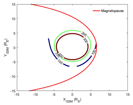
Figure 8. Equatorial GSM cuts of the TS04* modeled magnetosphere at the time of maximum compression. The red curve represents the location of the magnetopause boundary. The other colored lines represent the iso-contours of the local magnetic field strength over the 100–300 nT range.

permanently removing particles from the system. As previously mentioned, one of these processes can likely be the magnetopause shadowing (MS) in combination with outward radial transport, as suggested by the perfect match between the deep magnetopause incursion on sub-geostationary distances around 12:50 UTC of May 12 (Figure 6, panel a) and the abrupt ten-fold increment in solar wind dynamic pressure over the same time interval. Indeed, Gao et al. (2015) performed a POES/GOES/OMNI superposed epoch analysis of 193 relativistic-electron dropout events over 16 years, identifying the solar wind dynamic pressure and the north-south component of the interplanetary magnetic field as the main drivers of electron depletions in the ORB. In their study, while large solar wind dynamic pressure values are found to strongly push the magnetopause inward causing electrons to escape the magnetosphere, persistent southward interplanetary Bz,IMF preferentially results in electron scattering into the loss cone and consequent (wave-driven) precipitation to the atmosphere. Further, we have performed a TS04* simulation of the Earth’s magnetosphere at the exact time of minimum magnetopause distance, extracting X-Y GSM cuts that include the magnetopause location and the iso-contours of the local magnetic field strength over the 100–300 nT range (Figure 8). When MS is in action, ORB electrons are depleted on open drift paths that were previously closed (Kim et al., 2008; Turner et al., 2012). According to Sibeck et al. (1987) magnetic field iso-contours basically correspond to drift paths of equatorially mirroring (i.e., 90° pitch-angle) electrons that, at large L shell, are more likely to intercept the magnetopause and get lost. In Figure 8, the magnetopause intercepts the 100 nT line near the geosynchronous orbit at the time of maximum compression, which is strongly suggestive of MS having a role in removing relativistic electrons from the ORB. The dropouts observed by both MEPED-90° and HEPD-01 at relativistic energies penetrate down to L ∼ 4, which is a value significantly lower than minimum magnetopause standoff distance. A recent model (Ukhorskiy et al., 2015) suggests that MS and outward radial
transport should be sufficient to trigger such deep losses, even though this not rarely happens in concurrence with wave-induced precipitation to the atmosphere (Herrera et al., 2016). In addition, recent test-particle simulations in storm period (Ukhorskiy et al., 2006) address large diamagnetic effects from the enhancement of a partial ring current, which once again can result in violation of the third adiabatic invariant and prompt loss of ORB electrons to the magnetopause. The absence of long-lasting substorm activity completes the scenario, since earlier studies (Antonova et al., 2018; Jaynes et al., 2015) show a direct relationship between substorms and ORB electron replenishment during the storm’s recovery phase.

Finally, we detected a small Forbush decrease analyzing energetic protons at 500 km height. Though no clear two-step profile can be associated to this structure, the FD timing is consistent with an interplay between the IP shock and subsequent magnetic cloud as the origin of the small modulation, in accordance with earlier statistical surveys on the subject (Sanderson et al., 1990; Zhang & Burlaga, 1988).

As a closing comment, we want to highlight that despite the Sun is in general more active during its maximum and declining phases, recent papers showed the occurrence of extreme space weather events close to the solar activity minimum (Hayakawa et al., 2020; Hayakawa, Schlegel, et al., 2021; Piersanti et al., 2020). As a consequence, we remark that this kind of global analysis – namely, the study of an ICME propagation from its source on the Sun across the magnetosphere-ionosphere system to its impact in terms of magnetic field changes and magnetospheric particle redistribution, is still the straightforward way available to understand the complex dynamics of the processes occurring in the circumterrestrial environment from a space weather point of view. This analysis is an attempt to contribute to the systematization of the information available for these complex events, in the wider context of advancing our understanding of the aspects that determine the geoeffectiveness of solar activity manifestations.