
Mapping the South Atlantic Anomaly charged particle environmentwith the HEPD-01 detector on board the CSES-01 satellite
Table of Contents
- I. INTRODUCTION
- II. PARTICLE RATE MEASUREMENT WITH HEPD-01
- III. GEOGRAPHICAL CHARACTERIZATION OF THE SAA
- IV. INTEGRAL PARTICLE FLUX WITHIN THE SAA
- V. DISCUSSION AND CONCLUSIONS
- ACKNOWLEDGMENTS
- DATA AVAILABILITY
- APPENDIX A: RATE METER OVERFLOW CORRECTION
- APPENDIX B: ASSESSMENT OF SPACE WEATHER CONDITIONS
- APPENDIX C: SOURCES OF UNCERTAINTY AFFECTING FLUX ESTIMATION
- APPENDIX D: ANALYSIS OF THE T TRIGGER CONFIGURATION
I. INTRODUCTION
The geomagnetic field exhibits a region of notably smaller intensity, known as the South Atlantic Anomaly (SAA), extending for more than 80° in longitude and 40° in latitude above the southern Atlantic ocean. Within the SAA, the field intensity is lower by a factor ≳2 compared with the value at similar latitudes [1]. As a consequence, particles trapped in the geomagnetic field can reach lower altitudes, and the radiation environment within the SAA exhibits fluxes that are larger by 2–3 orders of magnitude with respect to neighboring regions. Particle measurements can complement magnetic ones to provide insight into the temporal evolution of the SAA [2], which makes up a privileged handle to study the dynamics of the geomagnetic field [3,4]. Moreover, the assessment of SAA particle fluxes is fundamental to studying perturbation phenomena such as geomagnetic storms, whereby an accurate estimate of the unperturbed, background population is necessary [5,6]. Furthermore, the knowledge of the SAA radiation environment is crucial for the design of space-crafts and devices that are expected to cross this region, both to prevent instrument faults and, in the case of manned missions, to safeguard astronaut health [7,8]. An empirical description of the trapped particle population around the Earth is provided, for example, by NASA’s AP9-AE9 models [9], which are routinely used to estimate the dose that a spacecraft receives during flight [10]. These kinds of models require updated measurements in order to keep up with the slow but constant evolution of the Earth’s magnetic field, especially from the perspective of an upcoming geomagnetic transition [1,3]. In the last two decades, the study of the purely geo-magnetic structure of the SAA [2,4,11] was paralleled by studies devoted to the investigation of its trapped particle content [8,12–14] and the validation of models [15]. Besides the measurement of particle fluxes within the SAA, a key feature that is typically investigated is the geographical drift of its center [13,14,16]. The High-Energy Particle Detector (HEPD-01) [17] on board the China Seismo-Electromagnetic Satellite (CSES-01) [18] is a valuable instrument to study the radiation environment within the SAA, being sensitive to electrons and protons with energy above a few MeV or few tens of MeV, respectively [19]. While the exceptionally high particle rate within the SAA hampers single-particle measurements, the instrument also provides count rate measurements under different trigger configurations that can be exploited to study some aspects of the SAA particle population. Since its commissioning, HEPD-01 has already provided insights into the SAA proton fluxes above 40 MeV [10,20]. The detector has proven to be an invaluable tool for low-energy cosmic ray [21,22] and space weather measurements, including the characterization of ground-level enhancements [23] and geomagnetic storms [24]. The aim of the present work is to provide the HEPD-01 characterization of the SAA particle content, by both investigating the spatial distribution of trapped particles and estimating the corresponding integral flux. While the SAA is foremost a magnetic phenomenon, the approach followed here is that of a purely particle-driven analysis. We consider rate meter data collected by HEPD-01 from 2018–2022 for different trigger configurations that correspond to different energy thresholds: from a fraction of an MeV to few tens of MeV for electrons, and from about 10 to 100 MeV for protons. We first map the particle rate within the SAA, analyzing day-night shifts and temporal drifts of the particle distribution. In particular, HEPD-01 measurement of the SAA drift is a valuable, independent result as it covers a temporal range for which assessments are scarce. Furthermore, narrowing the scope to the altitude and energy range of HEPD-01, it turns out that measurements are completely missing. Our results extend and enrich particle-based characterization of the SAA that, as stated above, are fundamental to complement geomagnetic-based measurements. We estimate integral proton fluxes that are compared—and show a good agreement—with the AP9 model predictions, validating it also at higher energies where the model itself is built by extrapolation. HEPD-01 rate meter data, along with the related pre-processing, are described in Sec. II. In Sec. III we analyze the spatial particle distribution around the maximum rate and its dependence on energy threshold, time, and day-night conditions. Thereupon, in Sec. IV we estimate the integral flux within this region and compare it with the AP9-AE9 model. Our findings are finally discussed in Sec. V in relation to the existing literature.
II. PARTICLE RATE MEASUREMENT WITH HEPD-01
HEPD-01 is hosted on the CSES-01 spacecraft, which orbits Sun-synchronously (97° inclination) at an altitude of approximately 500 km. The HEPD-01 trigger system uses different subsystems. An upper trigger plane “T” is made from an EJ-200 plastic scintillator layer segmented into six paddles, each of size 20 × 3 × 0.5 cm3, and readout relying on two photomultiplier tubes. In addition, below the trigger plane, HEPD-01 hosts a calorimeter made from a stack of 16 scintillator planes, each made of an EJ-200 plastic scintillator of size 15 × 15 × 1 cm3, and readout relying on two photomultiplier tubes [25,26]. The scintillator planes are henceforth referred to as Pn, with n 1⁄4 1; …; 16 (P1 is the uppermost one and P16 is the lowermost one). The data used in the present work consist of particle rates sampled at 1 s time resolution; no information on single-particle energy or particle type is acquired. Data correspond to five different trigger configurations, as shown in Table I, whereby each configuration is labeled with the corresponding logical operation between the T plane and one or more scintillator planes Pn. The effective areas for each trigger
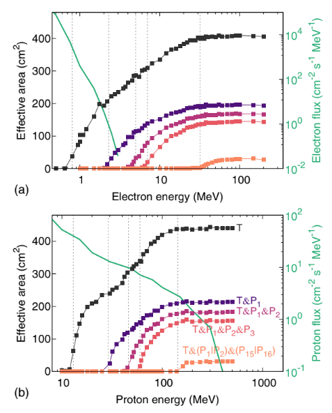
FIG. 1. Effective area of the different trigger configurations as a function of energy for electrons (a) and protons (b) obtained by means of Monte Carlo simulations. The configuration correspond- ing to each curve is reported in panel (b): the hue is darkest for the T trigger configuration, progressivelylighter for Tand P1, Tand P1 and P2, Tand P1 and P2 and P3, and the lightest is for Tand (P1 j P2) and (P15 j P16). The green solid lines without markers and corresponding ordinate axis on the right show the particle fluxes expected from the AP9-AE9 model at the center of the SAA. Gray dashed lines correspond to the effective thresholds reported in Table I.
configuration and for both electrons and protons, evaluated by means of Monte Carlo simulations, are shown in Fig. 1. Each trigger configuration is associated with an effective energy threshold—reported in Table I and shown in Fig. 1 by means of gray dashed lines—for both electrons and protons, which is evaluated as the minimum energy at which the corresponding effective area is above 10% of its maximum value.1 Finally, Table I also provides the maximum rate observed at the SAA center for each trigger configuration. In Fig. 1, the electron and proton fluxes provided by the AP9 AE9 model are also reported. According to such a
model, and by taking into account the effective area of the different configurations, the measured rates are expected to be dominated by the proton population for all configurations except the T one. Specifically, for the T and P1 configuration, the ratio between the rates of electrons and protons predicted by the AP9-AE9 model is 1.2 × 10⁻⁴. For the other trigger configurations, the same ratio is below 10−8. For this reason, in the following we refer to each trigger configuration, with the exception of the first one, by means of the corresponding energy thresholds for protons. The geographical coverage of the data is determined by the quasipolar, Sun-synchronous orbit of CSES-01. Each revolution around the Earth encompasses a curve in the latitude-longitude space, along which the local time at the satellite passage is ∼2 p. m. for descending semiorbits (henceforth “daytime”) and ∼2 a.m. for ascending semi- orbits (henceforth “nighttime”). Successive orbits “drift” westward in the longitudinal direction and return to approximately the same longitudinal position after about 5 days. Because HEPD-01 rate meter counters are implemented as 16-bit registers, raw data are affected by overflow artifacts whenever the trigger rate exceeds ∼65 kHz, a condition that—for the trigger configurations with lower energy thresholds—systematically occurs during passages over the poles and within the SAA due to the enhanced particle fluxes. These artifacts are corrected a posteriori, as described in Appendix A, thus allowing for a reliable measurement of rates up to several hundreds of kHz.
A. Particle rate maps
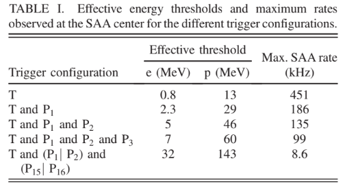
The first analysis step consists in constructing rate maps for each of the trigger configurations listed above, for both semiorbit conditions (daytime and nighttime) and different time intervals. Given a time interval Ik 1⁄4 1⁄2tk − δt; tk þ δtÞ centered at time tk and having a half-duration δt, all semiorbits of a given condition within Ik are initially considered. Because the aim of this work is to study unperturbed particle fluxes, we then exclude from the selection those data segments for which the space weather conditions, determined according to the description of Appendix B, are either “disturbed” or “stormy.” The excluded segments amount to approximately 36% of the overall data set. As a trade-off between the need to have sufficient statistics in building maps and the possibility to track temporal modulations, we consider nonoverlapping time periods Ik by setting a half-duration δt equal to 3 months and such that the central times tk are separated by 6 months. Accordingly, the first interval is centered at 2019-01-01 00∶00∶00 UTC and covers the span between 2018-10-02 00∶00∶00 UTC and 2019-04-01 23∶59∶59 UTC; the second is centered at 2019-07-02 00∶00∶00 UTC, and so on, until the last one centered at 2022-07-02 00∶00∶00 UTC. To build a map of particle rates, we consider a rectangular grid in latitude θ and longitude λ having 1° × 1° resolution. Because HEPD-01 is switched off in the polar regions at about jθj > 65°, we restrict maps to a reliable latitude interval given by −60° ≤ θ ≤ 60°. For a given grid cell labeled by i, j and centered at ðθi; λjÞ, a set of rate values frngði;jÞ is first collected by considering, for each semiorbit labeled by n, the average rate of data samples acquired when the satellite was inside the (i, j)th cell. Typically, this set contains around 8–10 values. Thereupon, the rate map value rˆi;j corresponding to the cell i, j is computed as the median of the frngði;jÞ set. The median is used to provide robustness against outliers. Because the satellite coverage of the latitude-longitude space is not complete at 1° resolution, cells for which a rate value is not available are filled by means of a spline interpolation over the neighboring cells placed at the same latitude. The interpolation is carried out by means of Steffen’s method [27], which ensures continuity up to the first derivative while guaranteeing that no spurious oscillations—and, therefore, no artificial maxima—are introduced. The resulting rate map ri;j does not have empty cells. Example rate maps ri;j for the trigger configurations T and T and P1, for the nighttime condition and related to the period centered at 2021-01-01 00∶00∶00 UTC, are shown in Fig. 2. In Fig. 2(a), which shows a map of rates that correspond to actual observations, the orbital footprint of the CSES-01 satellite is apparent. The corresponding map resulting from interpolation, by means of which the orbital gaps are filled, is shown in Fig. 2(b). Configuration T, which has the lowest energy threshold, measures particle rates spanning more than 3 orders of magnitude, from about 100 Hz in the equatorial region to about 400 kHz within the SAA and across the Van Allen belts.
III. GEOGRAPHICAL CHARACTERIZATION OF THE SAA
To assess the SAA position and shape from an interpolated rate map ri;j, we first compute in the latitude longitude plane a set of contour points ck 1⁄4 ðθk; λkÞ that bound the section of the SAA rate profile at half-maximum. The contouring algorithm is provided by the CountourPy
FIG. 2. Examples of maps ri;j for the T trigger configuration (a), (b) and the T and P1 one (c), built for the nighttime condition and during the 6-month period centered around 2021-01-01 00∶00∶00 UTC. Rates are represented via a logarithmic color scale. Latitudes above 60° and below −60° are excluded from the analysis. The map in (a) shows the measured data prior to interpolation, whose outcome is shown in (b).
library [28]. Each set ck contains ∼100 contour points. Thereupon, an ellipse, described by X2=a2 þ Y2=b2 1⁄4 1, where
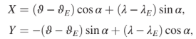
is fitted to the set of contour points ck; the fit parameters are the ellipse center coordinates θE, λE, the semiaxes a, b, and the angular tilt α between the ellipse “longitudinal” axis and the longitude direction. At the end of the procedure, we obtain a set of ellipse parameters for each trigger configuration, for each 6-month time period, and for each semiorbit condition (daytime or nighttime). The choice of an elliptical shape to fit the contour—besides requiring the relatively small number of five parameters—is a sound one: our purpose is to describe the section of a surface (the rate in the latitude-longitude space) in the proximity of its maximum, where the surface itself can be Taylor expanded to a paraboloid, whose sections are indeed ellipses. All ellipse fits provide a reduced chi-square significantly close to 1, given the number of fitted points ∼100. Moreover, we estimate the mismatch between the surface covered by each fitted ellipse and the surface enclosed by the polygon defined by the corresponding contour points. This mismatch turns out to be between 0.3% and 4%, with a median value of 1.1%. At fixed time and for a given semiorbit condition, the fitted ellipses for different trigger configurations, which correspond to different energy thresholds, exhibit a relative displacement. An example is shown in Fig. 3 for the time period centered at 2021-01-01 00∶00∶00 UTC and for both daytime and nighttime orbits. The displacement implies that the distribution of more energetic particles is shifted towards the northwest direction. Besides the energy dependence of the ellipse positions, a systematic shift between the ellipses associated with day-time and nighttime semiorbits is also apparent; in the example of Fig. 3, the nighttime ellipses, represented by dashed lines, appear to be shifted towards the south direction, with respect to their daytime counterparts. Such asymmetry, which is not accounted for by the uncertainty on the ellipses centers or the mismatch in the corresponding enclosed areas, could be explained in terms of the different geomagnetic field line configurations
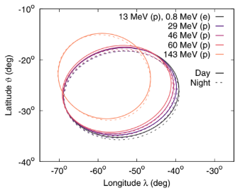
FIG. 3. Fitted ellipses on the SAA half-maximum contour for the time period centered at 2021-01-01 00∶00∶00 UTC and for both daytime and nighttime semiorbits. Each ellipse corresponds to a different trigger configuration and thus a different proton “(p)” and, for the first trigger configuration, electron “(e)” energy threshold, as reported in the figure key (the higher the energy, the lighter the hue). The two dashed ellipses with the lowest energy threshold (darkest hues) stem from the maps in Fig. 2.
on the day and night sides. By tracing both lines in the SAA region using the Tsyganenko and Sitnov model [29] under the quiet Solar wind condition, we evaluate the geographical position of the respective footprints. We find a difference in latitude of about 0.2°, caused by the action of the Solar wind which compresses the geomagnetic field lines on the day side and elongates them on the night side. In addition, we find a difference in longitude of about 0.5°, driven by the relative twisting of the field lines. These values are compatible with the observations found in Fig. 6 and are in agreement with theoretical models [30]. It is worth remarking that day-night differences of the SAA properties were found by analyzing electron fluxes [31]. Concerning the ellipse size and tilt, namely, the semiaxes a, b, and α, the different shapes in Fig. 3 suggest a dependence on energy—and, possibly, on semiorbit condition—as well. This dependence is displayed in Fig. 4 by taking the averages over all of the time periods of the semiaxes a, b and the tilt α. Because the “longitudinal” semiaxis a is always larger than the “latitudinal” semiaxis b, we henceforth identify a as the major semiaxis. Both semiaxes decrease monotonically with increasing energy, corresponding to a shrinking of the SAA extension for progressively more energetic particles. A discrepancy between daytime/nighttime conditions is essentially absent, with the exception of the highest-energy configuration, for which the semiaxes are larger during nighttime. It is worth highlighting that this observation does not necessarily correspond to a higher nighttime flux—as shown in the flux analysis of Sec. IVA—but rather to a broader geographical distribution. Besides the daytime/nighttime
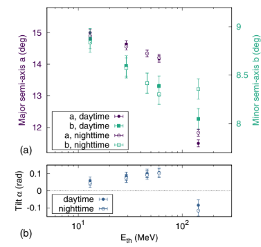
FIG. 4. (a) Dependence on energy and semiorbit condition of the ellipses semiaxes a, b. The points corresponding to the minor semiaxis b are referred to the right ordinate axis, as highlighted by the colored labels. (b) Dependence on energy and semiorbit condition of the angular tilt α.
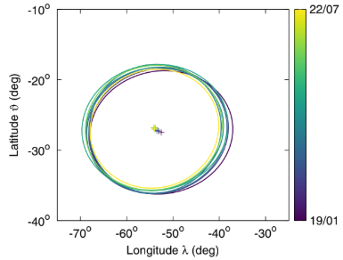
FIG. 5. SAA ellipse evolution over time for the T trigger configuration and nighttime condition. The color scale represents the central time of each time interval, from 2019-01-01 00∶00∶00 UTC to 2022-07-02 00∶00∶00 UTC.
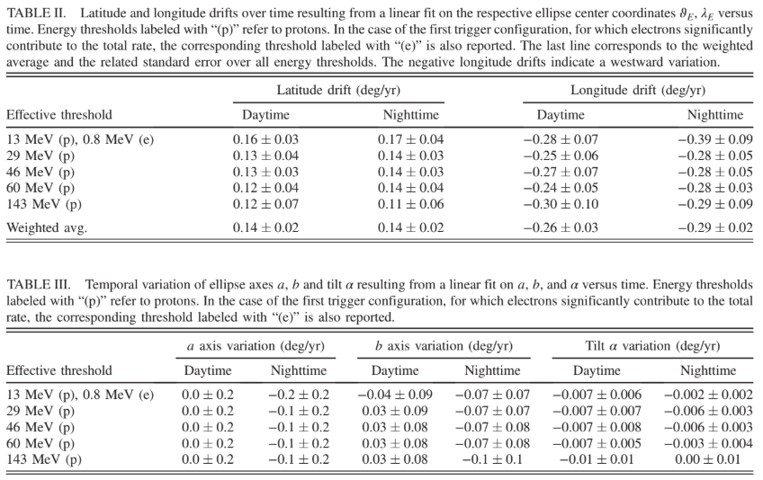
difference, the highest-energy configuration is also peculiar because of the corresponding negative tilt (α < 0).Over the 4 years analyzed here, a temporal drift of the SAA location is observed. An example at a fixed energy threshold and condition, namely, the T trigger configuration for nighttime semiorbits, is shown in Fig. 5, exhibiting an apparent northwest drift over time. The coordinatesðθE; λEÞ of the ellipse center for different trigger configurations, time periods, and semiorbit conditions are shown in Fig. 6. The figure provides a summary of
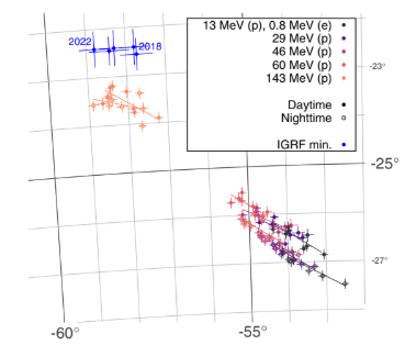
FIG. 6. SAA ellipse center coordinates for different time periods, semiorbit conditions, and energy thresholds, as reported in the figure key, within the analyzed epoch 2018–2022. The minimum of the geomagnetic field according to the IGRF model is also shown for the years 2018–2022 (topmost points). For all data points, time proceeds from right to left. To more faithfully represent the relative
latitudinal and longitudinal displacements, the map is displayed by means of an equidistant conic projection (standard parallels: −10° and −40°; origin: λ0 1⁄4 −50°, θ0 1⁄4 −30°) [32].
evidence of a time dependence was found. Specifically, for each trigger configuration and semiorbit condition we evaluate the Pearson correlation coefficient between time and either a, b or α. All evaluations provided—under the null hypothesis of normal uncorrelated variables—p-values larger than 0.07, leading to the conclusion that the hypothesis of uncorrelated variables cannot be rejected. Furthermore, again for each trigger configuration and semiorbit condition, linear fits of either a, b, or α versus time yield slopes compatible with zero within 2 standard deviations in all cases (the p-values of the corresponding chi-square tests are all above 0.01 except for two cases out of 30). This last result, namely, the fitted slope of the temporal variation for the ellipse semiaxes and tilt, is shown in Table III. As mentioned above, all slopes are compatible with zero, leading to the conclusion that a time dependence of the ellipse semiaxis or tilt is either absent or too small to be significantly detected within the time period considered here.
IV. INTEGRAL PARTICLE FLUX WITHIN THE SAA
The rate meter data analyzed in the present work do not provide a measurement of particle energy; rather, the input
particle flux is integrated over the whole energy range accessible by each trigger configuration. Nevertheless, by introducing an assumption about the spectral information, namely, the functional form of the energy dependence of the flux, we are able to provide an estimate of the integral flux above a certain energy threshold. The spectral information is extracted from the AP9-AE9 models of trapped particles [9]. For a given trigger configuration, the measured rate can be expressed as
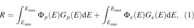
where ΦαðEÞ and GαðEÞ are the differential flux and effective area, respectively, associated with the species α, namely, α 1⁄4 p for protons and α 1⁄4 e for electrons. The integration bounds Emin, Emax—which in principle would be 0, ∞—are actually determined by the fact that GαðEÞ and ΦαðEÞ vanish, respectively, below or above a given energy. Specifically, the lower bound is effectively set by the minimum energy above which the estimated effective area is nonzero, GαðEÞ > 0 (see Fig. 1). On the upper side, instead, we integrate up to the maximum energy for which a nonvanishing value ΦαðEÞ > 0 of the flux is provided by the AP9-AE9 model, namely, 400 MeV for protons and 3 MeV for electrons. These limits set by the model are justified by the fact that proton and electron fluxes decrease steeply with increasing energy, as one can see in Fig. 1. To provide numerical references, the proton flux decreases by a factor ∼3 × 10² between 5 and 300 MeV, from ∼200=cm2 s MeV to ∼0.7=cm2 s MeV; the electron flux decreases more dramatically by a factor ∼106 between 0.5 and 3 MeV, from ∼105=cm2 s MeV to ∼0.05=cm2 s MeV. In principle, the observed rate is contributed by both electrons and protons. As already mentioned in Sec. II, by computing the rates expected a priori according to the AP9-AE9 model, one finds out that in the case of the T trigger configuration both the electron and proton contributions to the rate R are relevant. Conversely, for all other trigger configurations, the energy threshold for electrons is sufficiently high so as to make the electron flux contribution negligible (see also Fig. 1). Consequently, for all configurations except the T one, the above expression for R can be reduced to the first integral term only. The procedure followed here is to assume a functional dependence φαðEÞ of flux on energy and provide estimates of its energy-independent scale constant Fα. In other words, we assume
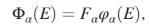
where the function φαðEÞ is defined so that
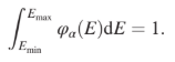
Assuming that φeðEÞ, φpðEÞ are given, the integrals in Eq. (1) are numerically computed, yielding the coefficients Γα 1⁄4 R Emax Emin φαðEÞGαðEÞdE. In the case of the T trigger configuration, the rate can then be expressed as R 1⁄4 FpΓp þ FeΓe. On the other hand, as explained above, in the case of the other trigger configurations the expression simplifies to R 1⁄4 FpΓp. In the present work, the shapes φeðEÞ, φpðEÞ are computed from the AP9-AE9 model by extracting the omnidirectional fluxes corresponding to the SAA center and normalizing them by their respective integrals. The effective areas GeðEÞ, GpðEÞ are those shown in Fig. 1 and computed via Monte Carlo simulations. The estimation of the integral flux is carried out by considering the maximum of the rate map within the SAA region. It is worth recalling that rate maps are built by considering the median value of the rate within each cell; consequently, the information extracted from the AP9-AE9 model is that of the median flux. Given these quantities, for each trigger configuration, we thus provide either a linear constraint between the flux scale constants Fe, Fp (T trigger configuration) or a direct estimate of the proton flux scale constant Fp (other trigger configurations). The sources of uncertainty affecting the flux estimation are discussed in AppendixC. Henceforth, errors are reported as the quadrature sum of statistical and systematic contributions. Concerning the AP9-AE9 model, we report two values for the uncertainty, referred to as “local fluctuations” and “geographic variability,” as explained in Appendix C.
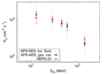
FIG. 7. Integral proton flux Ψp above a given energy threshold averaged over all time periods and conditions. The values estimated out of HEPD-01 data (red filled circles) are compared with those computed using the AP9-AE9 model (black squares). Error bars correspond to the minimum and maximum among all 6-month period estimates. Each red data point is contributed by the rate measured by one trigger configuration, whose correspondence to the energy threshold is reported in Table I.
A. Integral flux and comparison
with AP9-AE9 model
The outcome of the present analysis is given by a set of estimated F cp values, each one associated with a trigger configuration. In the case of the T trigger configuration, Fcp is evaluated out of the linear constraint between Fe, Fp, as explained in Appendix D. In principle, one could directly compare the estimated Fcp values with the same parameter extracted from the AP9-AE9 model. However, while Fp
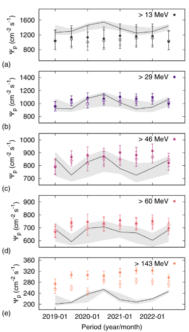
FIG. 8. Integral proton flux Ψp as a function of the time period. Each panel corresponds to a different trigger configuration, and therefore a different proton energy threshold: (a) 13 MeV, (b) 29 MeV, (c) 46 MeV, (d) 60 MeV, and (e) 143 MeV. Filled and empty points correspond to daytime and nighttime con- ditions, respectively. The solid lines and shaded areas are the AP9 estimates and the related geographical variabilities (black dots and error bars in Fig. 7). The lowest-energy evaluation is carried out by removing the electron contribution to the rate, as explained in Appendix D.
has a well-defined meaning, its physical interpretation in terms of particle fluxes is not immediate. Therefore, we instead compute the integral proton flux above a given energy threshold, namely,
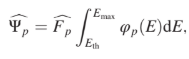
whereEth is the energythreshold. Similarly, the flux predicted by the model is assessed as Ψp 1⁄4R Emax Eth ΦpðEÞdE. Each energy threshold Eth corresponds to a single trigger configuration, and the corresponding Eth values are those reported in Table I. Accordingly, each Ψcp value computed as described above is contributed by the rate measured by a single trigger configuration. Figure 7 shows the estimated integral flux and its comparison with the AP9-AE9 model predictions. The estimate is first carried out separately over each time period and condition; because no significant time modulation is observed (see below), the data of Fig. 7 are computed as the average over the set of estimates, while error bars are assessed as the minimum and maximum extents reached by the errors of the single evaluations. The estimates provided by HEPD-01 are in agreement with the model predictions, even by considering only the uncertainty due to the geographic variability. A breakdown of the flux estimates for each time period and condition is finally displayed in Fig. 8. Even in this case, the estimated integral fluxes are mostly compatible with the AP9 model predictions, with the exception of the case of the highest-energy threshold of Fig. 8(e). In that case, the estimate provided by HEPD-01 is systematically larger than the prediction by up to 50%.
V. DISCUSSION AND CONCLUSIONS
Data collected by the HEPD-01 rate meter under different trigger configurations proved to be a valuable asset to map the populations of trapped particles in the Earth’s magnetosphere, covering more than 3 orders of magnitude in particle rate at the lowest energy threshold (see Fig. 2). This capability allowed us to assess the drift of the SAA center in the 2018–2022 period, which moves—consistently across energy thresholds—northward by ð0.14 0.02Þ deg =yr and westward by ð0.28 0.02Þ deg =yr. Our drift estimate is compatible with several previous assessments reported in the literature, based on satellite observations at different altitudes with different instruments, and covering the last three decades [12]. For example, by relying on the Defense Meteorological Satellite Program (DMSP), whose multiple spacecrafts enable long-term temporal coverage, a northward drift of ð0.16 0.09Þ deg =yr and westward drift of ð0.36 0.06Þ deg =yr [37] was assessed by considering particle noise pulses attributed to >45 MeV protons within an ultraviolet imager. An estimate of the drift on the same set of satellites, though using a particle spectrometer, provided similar values: 0.06 deg =yr northward and 0.28 deg =yr westward [14]. Larger northward and westward drifts, respectively, ð0.17 0.01Þ deg =yr and ð0.43 0.01Þ deg =yr, were observed by analyzing rates in the 1–250 keV range collected in the time span 2017–2019 by the particle monitors onboard the Insight-HXMT satellite, flying at ∼550 km [38]. The SAA was also characterized by measurements that do not rely on particle detection; for example, a similar drift of 0.12 deg =yr northward and 0.24 deg =yr westward was estimated by optical radiance (near-infrared and visible) measurements from the Along Track Scanning Radiometer onboard the ERS-1, ERS-2, and ENVISAT ESA satellites, flying at 800 km [39]. The above list of drift values is not exhaustive and tables collecting different assessments of the SAA drift are reported, for example, in Refs. [37,38]. It is worth remarking that occasionally drift values present in the literature are not compatible with others and with the present ones; discrepancies might be conceivably attributed to different altitudes, time periods, instrumentation, and measurement of observables other than particles. Nevertheless, there seems to be a general consensus on a westward and northward drift of approximately 0.3 deg =yr west and 0.1 deg =yr north. An exception is provided by the analysis of the Low-Energy Ion Composition Analyzer sensor on board the SAMPEX spacecraft flying at ∼600 km. The corresponding SAA integral rates (mostly protons > 10 MeV and electrons > 0.6 MeV) were used to estimate a westward drift of ð0.20 0.04Þ deg =yr alongside a southward drift of ð0.11 0.01Þ deg =yr [34]. This latter result is reversed with respect to the previously cited latitudinal drifts; considering that the geomagnetic field evolution is not uniform in time [40], this observation highlights the need for updated measurements of the SAA properties, covering longer epochs and obtained through different instruments. No temporal variations of the ellipse parameters a, b, α, which describe the profile of the SAA central region, were found. This implies that, if any such variation exists, its extent is below our capability to detect it, which is primarily limited by the spatial resolution of the used grid. The availability of rate measurements at different energy thresholds allowed us to outline the energy profile of trapped particles within the SAA (see Figs. 3 and 6). The locations of the maximum rate for more energetic particles are progressively shifted towards the northwest up to the highest-energy (>143 MeV) population of protons that appears shifted by 3° north and 4° west with respect to the lowest-energy population. It is worth remarking that, as shown in Fig. 6, particle-based assessments of the SAA center are displaced with respect to the minimum of the geomagnetic field, here evaluated by relying on the IGRF model. Moreover, the higher the particle energy, the closer the particle-based SAA center—and thus the particle flux maximum—to the minimum of the geomagnetic field. This effect is indeed expected according to numerical calculations [16] as well as previous measurements of particle fluxes by the SAMPEX [34], NOAA [35], and DMSP satellites [14], whereby maximum particle fluxes are systematically shifted towards the southeast with respect to IGRF field minima. The integral proton flux estimated from HEPD-01 data is in agreement with the AP9 model, thus proving their potential to become a valuable input to improved models of trapped particles. A significant discrepancy is observed only in the highest-energy trigger configuration [see Fig. 8(e)]. This difference might be due to the fact that, above≳200 MeV, the AP9 model flux is built through extrapolation due to the lack of higher-energy data [9]. Additionally, above these energies, contributions from cosmic-ray protons with momentum exceeding the rigidity cutoff are expected. These contributions are not accounted for by the models and thus might explain the observed excess. Over the 4 years analyzed here, no significant seasonal effect on the flux was found. Moreover, we did not observe a significant particle flux variation over time such as that observed by PAMELA [41] which, however, covered an 8-year period and a proton energy range (80 MeV–2 GeV) that only marginally overlaps with that of HEPD-01. The present characterization of the SAA enriches the observations of the related radiation environment in the proton energy range above ≳13 MeV. The HEPD-01 estimate of the integral proton flux provides a validation of the AP9 model, while the observed SAA drift towards the northwest direction extends the experimental evidence on the evolution of the geomagnetic field, which is crucial for models of its temporal evolution, to the 2018–2022 period, for which particle-based assessments of the SAA drift are almost absent and are complemented by the present one [40]. HEPD-02, an improved version of the detector that is expected to be launched on board CSES-02 by the end of 2024 [42], will access a wider range of particle energy and, by virtue of prescalers that will remove any saturation issue, will be able to concurrently measure particle energies on multiple masks [43]. Therefore, HEPD-02 will allow to further refine and extend the present characterization of the SAA, providing energy-resolved estimates of fluxes.
ACKNOWLEDGMENTS
This work makes use of data from the CSES mission, a project funded by the China National Space Administration (CNSA), China Earthquake Administration (CEA) in collaboration with the Italian Space Agency (ASI), National Institute for Nuclear Physics (INFN), Institute for Applied Physics (IFAC-CNR), and Institute for Space Astrophysics and Planetology (INAF-IAPS). This work was supported by the Italian Space Agency in the framework of the “Accordo Attuativo 2020-32.HH.0 Limadou Scienza+” (CUP F19C20000110005), the ASI-INFN Agreement No. 2014-037-R.0, addendum 2014-037-R-1-2017, and the ASI-INFN Agreement No. 2021-43-HH.0.
DATA AVAILABILITY
The data that support the findings of this article are not publicly available. The data are available from the authors upon reasonable request.
APPENDIX A: RATE METER OVERFLOW CORRECTION
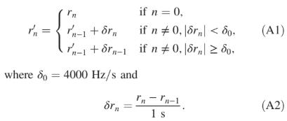
As introduced in Sec. II, rate meter counters on board HEPD-01 undergo overflows for rates exceeding 216 Hz ≃ 65 kHz, leading to jump-like artifacts in the rate time series. An example of this issue is shown in Fig. 9. Overflows are mostly observed for the trigger configurations with the lowest energy threshold and occur when the satellite is crossing the SAA and the Van Allen belts. To correct for this effect, we developed a correction algorithm that acts on segments of each semiorbit that can potentially be affected by overflows; these segments are
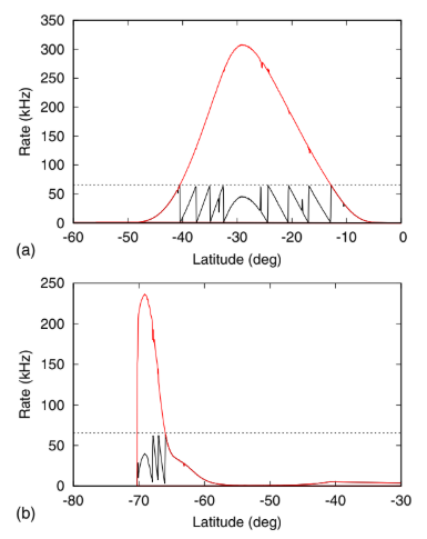
FIG. 9. Example of the overflow correction algorithm applied to the rate measured by the T trigger configuration within segments of orbit crossing (a) the SAA or (b) the southern hemisphere belts. Black solid lines correspond to raw rates, while red lines, which overcome the dotted horizontal lines, result from the correction. Dotted lines correspond to the overflow limit of 216 Hz.
defined so as to fully contain either the SAA or the belts of the northern or southern hemispheres. Outside of these regions, the measured rate is well below the overflow limit and the resulting time series do not show the issue. As a first step, within a segment, the correction algorithm attempts a reconstruction of the actual rate by integrating its (numerical) time derivative, neglecting those samples for which the derivative is suspiciously large. More specifically, the reconstructed rate r0 n at sample n of the segment is computed using the measured rate rn according to
The reconstruction is carried out both in the forward direction n 1⁄4 1; …; N, where N is the number of samples within the segment, and in the backward direction, obtained by recasting n → N − n þ 1. For each nth sample, we retain the largest between the two values of r0 n obtained through the forward and backward reconstructions. In the second step, the algorithm compares the reconstructed rate r0 n with the measured one rn: if the difference overcomes 215, namely, half of the overflow limit, the rate is corrected according to
where ⌈xc is the closest integer to x. As a last step, “glitches” in the reconstructed data corresponding to sudden increases or decreases of the rate and affecting a single sample—which are spurious effects due to “jumps” in the raw data—are corrected by replacing the corresponding value with a linear interpolation of the neighboring samples. Two representative examples of the results of the over-flow correction algorithm are shown in Fig. 9 for two orbit segments: one crossing the SAA and one crossing the belts. These examples uphold the reliability of the overflow correction algorithm. Occasionally, when the particle rate changes abruptly (approximately above 20 kHz=s or, equivalently, 300 kHz= deg in latitude), a correct reconstruction of the true rate is unfeasible. This issue occurs exclusively in the belts and thus does not affect the SAA assessment. Moreover, the choice of computing the median rate observed in each map cell provides robustness against these occasional artifacts.
APPENDIX B: ASSESSMENT OF SPACE WEATHER CONDITIONS
To avoid introducing bias in the determination of particle fluxes due to external perturbations, we assess space weather conditions by relying on the SYM-H index. Specifically, we download raw SYM-H data from the OMNIWeb database [44], where the index was extracted with 1 minute resolution. The index was then averaged over consecutive, nonoverlapping time intervals of 3 hours. For each interval labeled by i, the space weather conditions were determined from the averaged SYM-H index Si according to the following rule [45]: “quiet” intervals correspond to −10 < Si ≤ 10; “disturbed” intervals corre- spond to −40 < Si ≤ −10; “stormy” intervals correspond to any other value, namely, Si ≤ −40 or Si > 10. The present classification is coherent with those found in the literature and it is possibly more conservative [46,47]. Intervals for which the condition was not deemed to be “quiet” were excluded from all analyses discussed in the present work. The selection also mitigates the presence of abrupt changes in rate that would lead the overflow correction algorithm astray.
APPENDIX C: SOURCES OF UNCERTAINTY AFFECTING FLUX ESTIMATION
The estimation of the flux scale constants Fe, Fp is affected by the statistical uncertainty on the median rate R, which is typically of the order of 3%. Moreover, a systematic uncertainty linked to the effective areas GeðEÞ, GpðEÞ has to be taken into account. To this purpose, the evaluation of the effective areas using Monte Carlo simulations was carried out under different settings of the energy deposition thresholds required to activate trigger and scintillator planes. The variability of the effective areas resulting from different energy thresholds results in an error in the Γe, Γp coefficients. Such error, which was assumed as the systematic uncertainty due to the uncertainty on the effective area, turns out to be of order 2%. An exception is provided by the T trigger configuration for electrons; in that case, because the electron flux varies by 4 orders of magnitude between 1–3 MeV, even slight variations of GeðEÞ in that range yield variations in Γe that are as large as 15%. A systematic uncertainty should also be attributed to the possible error in estimating the flux functional shapes φeðEÞ, φpðEÞ from the AP9-AE9 model. This uncertaintycan be evaluated by considering the variability of flux shapes provided by the model in a region around the SAA center—in this case, a 2° disk in the latitude-longitude space—and, again, by translating this variability into a relative error on the Γe, Γp coefficients. This relative error is of order 5%. As far as the error on the AP9-AE9 model fluxes is concerned, we consider here two kinds of uncertainties, which convey two different kinds of information on the model variability: “local fluctuations” and “geographic variability.” With regard to the local fluctuations, the AP9-AE9 model provides, in addition to the median flux, percentile values; in the following, we consider the 15th and 85th percentiles, approximately corresponding to a 1σ interval in the case of normal variables. On the other hand, one can consider the variability of the median flux due to uncertainty in the geographic location at which it is estimated. We therefore evaluated the maximum and minimum fluxb in a circular region of 2° around the estimation location: the two values define the asymmetric error bar due to the aforementioned geographic variability.
APPENDIX D: ANALYSIS OF THE T TRIGGER CONFIGURATION
The constraint on Fe, Fp derived from rate data for the T configuration, expressed in the form
corresponds to a straight line in the Fp, Fe plane. An example of this line, along with the related uncertainty, is shown in Fig. 10, which refers to the time interval centered at 2021-01-01 00∶00∶00 UTC and the nighttime condition. The values and uncertainty of Fp, Fe provided by the AP9-AE9 model are also shown in the figure. The constraint obtained in the present work is in agreement with the model. As mentioned above, because the analysis for the otherbtrigger configuration provides a direct estimate of the proton flux scale constant F cp, we exploit our constraintto also provide a similar estimate on the same parameter for the T trigger configuration. To this purpose, we assume the

FIG. 10. Plot of the Fp, Fe relation derived from the rate data of the T trigger configuration for the nighttime condition of the time interval centered at 2021-01-01 00∶00∶00 UTC. The blue solid line corresponds to the linear relation obtained from the rate data, while the offsets of the dashed lines with respect to the solid line correspond to the related uncertainty. The black point provides the values of Fp, Fe computed using the median fluxes from the AP9-AE9 model, with the related geographical variability in black and local fluctuations in gray. The red cross and shaded area provide—once Fe is assumed from the model—HEPD-01’s
estimate of Fp.
value Fe from the AP9-AE9 model (ordinate of the black point in Fig. 10) and consequently obtain an F cp value as the abscissa at which the constraint matches the assumed value of Fe (red cross in Fig. 10). The uncertainty related to this F cp estimate is promptly given by considering the maximum extent, along the Fp direction, of the uncertainty on the constraint line, namely, the red shaded area in Fig. 10; the height of the shaded area is given by the uncertainty on the Fe value (as provided by the model).